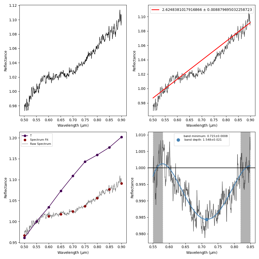
Pipeline for Visible Spectra

Out:

           slope  slope_unc tax  ... depth_unc  center  center_unc
000752  2.624838    0.00888   T  ...     0.021   0.715      0.0008

[1 rows x 8 columns]

import cana

# First load an spectrum
# you can do: spec = cana.loadspec('path to your spectrum file')

# For the example, we will just gonna use one from the available datasets.

spec = cana.datasets.getspectrum('000752', ref='primass')

# Defining parameters that will be used in the pipeline
# We are explicitating here, but all values above are actually set as default
# and can simply be setted as params='default'

# The Slope method
# Defaults: wmin=0.4, wmax=0.9, norm=0.55, errormethod='rms',
#           error_param=None, montecarlo=1000, speckwargs=None
slope = cana.Slope()

# The Taxonomy method
# Defaults: system='demeo', method='chisquared', return_n=3, norm=0.55,
#             fitspec=True, speckwargs=None
tax = cana.Taxonomy()

# The band method
# Defaults: lowerwindow=0.04, upperwindow=0.04
continuum = cana.Continuum(lowerwindow=0.03, upperwindow=0.03)

# Depth Defults: wmin=0.54, wmax=0.88, continuum=Continuum()
band = cana.Depth(wmin=0.55, wmax=0.85, continuum=continuum)

isband = {'min_depth': 1, 'theoric_min': 0.7,
          'max_dist': 0.5, 'sigma': 3}

# Running the pipeline
# if spec is a list of spectra path, outplot can be setted as
# a directory to save the plots
# Defaults: params='default', error=SpecError(),
#                      isband=None, speckwargs=None, outplot=None,
#                      verbose=False
pipe = cana.primitive_visible(spec, params=[slope, tax, band],isband=isband, outplot='show')

# Printing results
print(pipe)